[Study Notes] Meta Learning and MAML

This blog summarizes my notes on meta-learning and one of the classical meta-learning strategies, Model-Agnostic Meta-Learning (MAML) [1], covering its motivation, methodology, and experiments. I appreciate the online course by Hung-yi Lee [2] for providing a comprehensive overview of meta-learning.

1. Challenges in bioinformatics and chemical informatics problems

Traditional machine learning models require large amounts of data for specific tasks, which isn't feasible for all problems. For instance, in bioinformatics and chemical informatics, we often encounter various experimental conditions that may come from different groups or different projects. However, for each condition, we may have only a small amount of data due to limitations in labor, budget, and time. Meta-learning can potentially address these challenges by training models to quickly adapt to new tasks with minimal data.

2. What is Meta-Learning?

Meta-learning, often referred to as "learning to learn," is an approach that not only learns the model parameters \(f_\theta\) but also the training algorithm \(F_\phi\) as shown in the following figure.

To achieve this goal, multiple tasks are needed for meta-learning. These tasks are divided into training tasks (e.g., task 1 and task 2 in the figure above) and test tasks. During training, components of learning algorithms are learned across training tasks. Evaluating meta-learning methods involves training models on test tasks, which differs significantly from traditional machine learning methods.

It's important to note that meta-learning is not the same as few-shot learning. While few-shot learning involves using a small amount of data to train a model, meta-learning enables training a model on limited data by training it across multiple tasks.

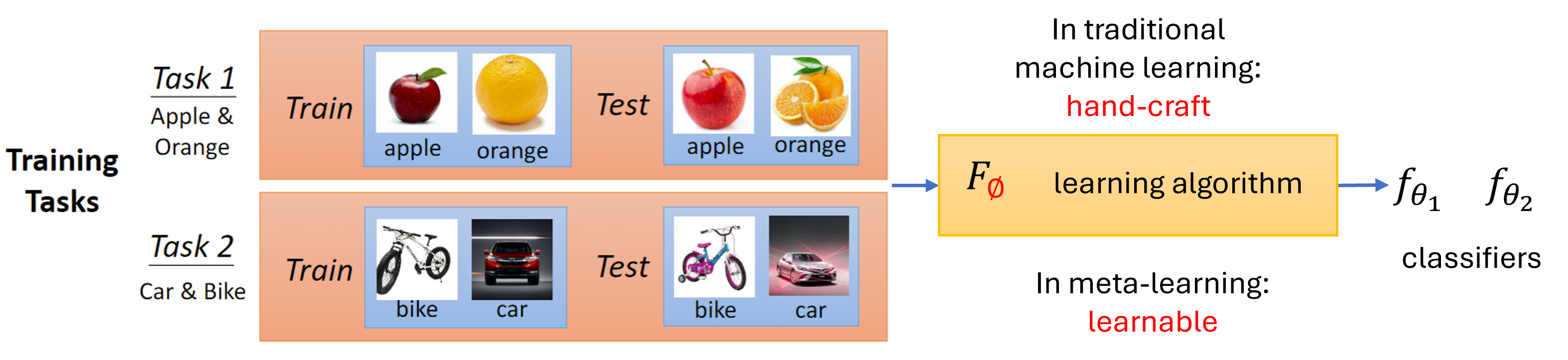
Various components in a learning algorithm can be learned, including:

• Data preprocessing: Differentiable automatic data augmentation [3]; Meta-weight-net: Learning an explicit mapping for sample weighting [4]
• Model architecture: Network architecture search [5]
• Optimizer (learning rates): Learning to learn by gradient descent by gradient descent [6]
• Initialized parameters: Model-Agnostic Meta-Learning (MAML) [1]

3. Model-Agnostic Meta-Learning (MAML)

3.1 Methodology

Let's refresh the aim of MAML that we wanna find an initialized weights \(\phi\) that when applying on test tasks, the model could perform well. Then the loss function for MAML can be defined as follows: \[ L(\phi) = \sum^N_{n=1}l^n(\hat{\theta}^n) \] where \(\phi\) represents the model's initial weights, \(\hat{\theta}^n\) represents the model's weights learned from task \(n\), and \(l^n(\hat{\theta}^n)\) is the loss on the test set of task \(n\).

The model's weights \(\hat{\theta}^n\) can be learned through gradient descent as traditional machine learning does. We always constrain it as a one-step gradient update: \[ \hat{\theta}^n = \phi - \alpha {\nabla}_{\phi}l^n(\phi) \] where \(\alpha\) is the learning rate.

How can we minimize \(L(\phi)\)? Gradient descent! \[ \phi \leftarrow \phi - \beta {\nabla}_{\phi}L(\phi) \] where \(\beta\) is the learning rate for the meta-learner.

Since we already have the definition of \(L(\phi)\), we can replace it in the previous equation: \[ \phi \leftarrow \phi - \beta {\nabla}_{\phi}\sum^N_{n=1}l^n(\hat{\theta}^n) \] Using a one-step gradient update to train the model's parameter \(\hat{\theta}^n\), we arrive at the final update rule for MAML: \[ \phi \leftarrow \phi - \beta {\nabla}_{\phi}\sum^N_{n=1}l^n(\colorbox{yellow}{$\phi - \alpha {\nabla}_{\phi}l^n(\phi)$}) \] We refer to the yellow part as the inner loop and the entire process as the outer loop. Typically, we split the data from training tasks into two parts: one for the inner loop and the other for the outer loop. Since the inner loop is a one-step gradient update, it is computationally efficient and requires fewer data points; it can even be performed using \(k\)-shot learning.

3.2 MAML vs. Pretraining

As both MAML and pretraining aim to find a good initialization for the model, what is the difference between them?

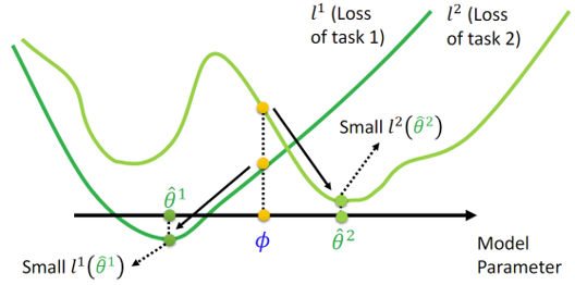
In MAML, the goal is to find \(\phi\) that achieves good performance after training, expressed as: \[ L(\phi) = \sum^N_{n=1}l^n(\hat{\theta}^n) \] As shown in the figure below, through MAML, we can find initialized weights \(\phi\) that perform well after fine-tuning, even if \(\phi\) does not achieve the best performance initially.

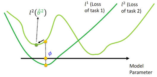
In contrast, pretraining focuses on finding \(\phi\) that achieves good performance without training specific tasks: \[ L(\phi) = \sum^N_{n=1}l^n(\phi) \] In the figure below, \(\phi\) initially performs well on both task \(1\) and task \(2\), but after fine-tuning, \(l^2(\hat{\theta}^2)\) converges to a locally optimized point, which is not as optimal as the result achieved by MAML.

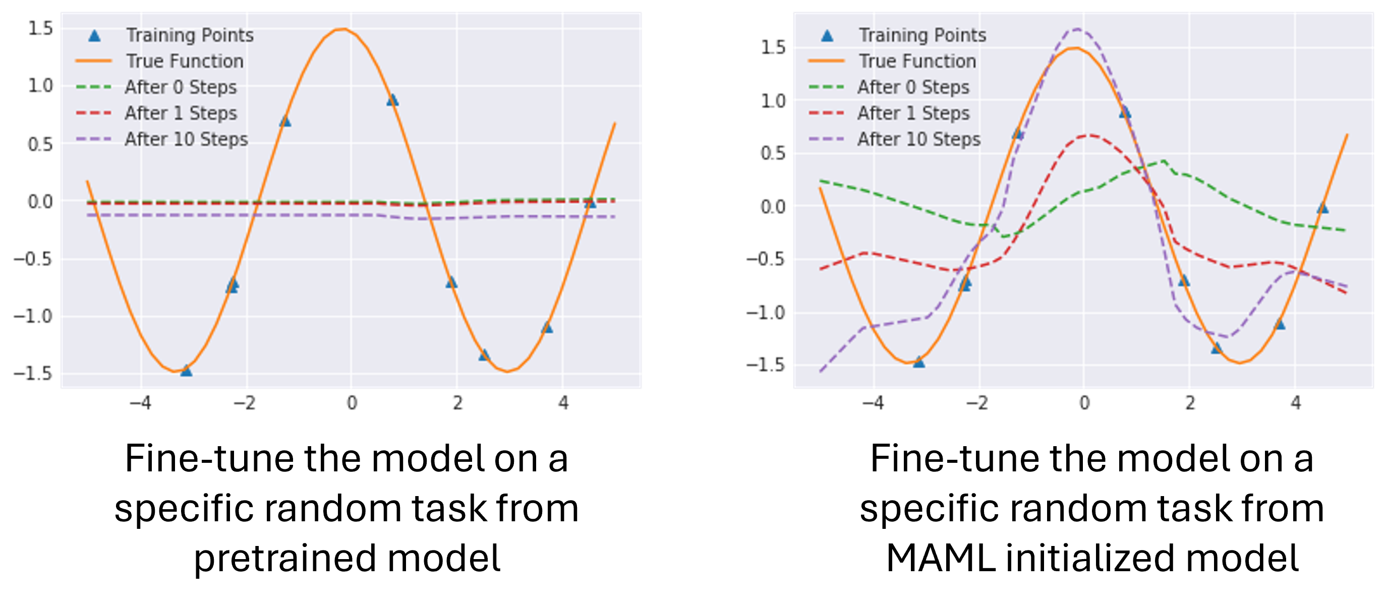
3.3 Experiments: regression on Sine wave

In a toy example, we define a task \(y = a sin(x + b)\). We sample \(k\) points from the target function to estimate it, The tasks are formed by sampling \(a\) and \(b\).

The following figures show the randomly generated 3 and 1000 tasks, respectively. You may already notice the problem: if we train a model on all 1000 tasks together, it would converge to the average of all tasks, which is zero.

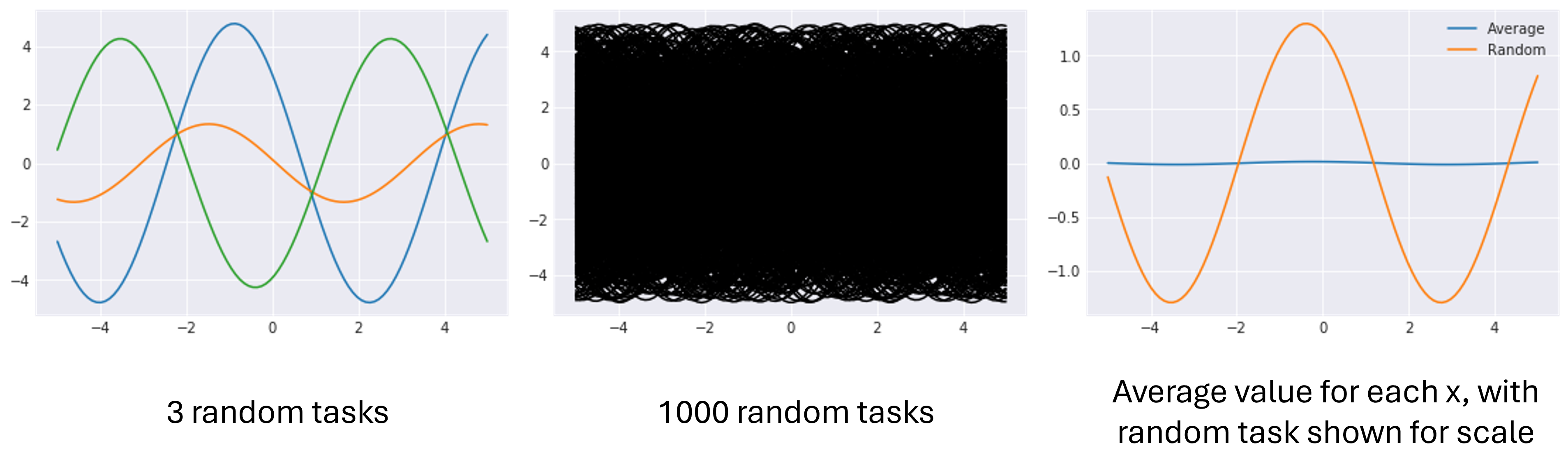
Incidentally, this is a toy example to illustrate the issue clearly. In real-world applications, this problem may not be as obvious. However, the key takeaway is that when training a model on multiple tasks, we need to consider whether the diversity of tasks negatively impacts individual task performance.

The following figures show the performance of fine-tuning models from MAML and pretraining on sine wave simulation. As we expected, the pretrained model is initialized at all zeros. After fine-tuning on 10 instances, it cannot converge. However, the model initialized by MAML does converge.

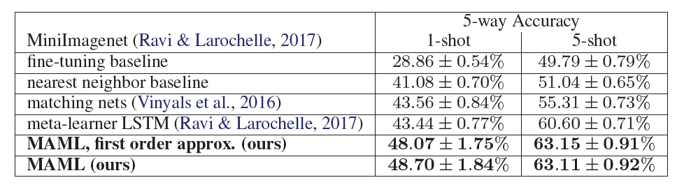
3.4 Experiments: classification

The authors took \(5\)-way \(1\)-shot and \(5\)-way \(5\)-shot evaluations on MiniImagenet dataset. This dataset is commonly used as a few-shot learning benchmark, involving 52 classes. The \(N\)-way classification problem is set up by selecting \(N\) unseen classes and providing \(K\) instances of each class. The model is then fine-tuned on these instances to classify the remaining instances from those classes.

Following Works

MAML marks the start of meta-learning for initialization. It faces challenges such as sensitivity to task diversity, dependence on adequate training tasks, and difficulties in scaling to complex models. Subsequent research efforts aim to address these issues:

• [ANIL, Almost No Inner Loop] Rapid learning or feature reuse? Towards understanding the effectiveness of MAML [8].
• [MAML++] How to train your MAML [9].
• [Reptile] On first-order meta-learning algorithms [10]. For more information, visit OpenAI's Reptile page.

References

1. Finn, C., et al. (2017). Model-agnostic meta-learning for fast adaptation of deep networks. ICML
2. Hungyi, L. (2021). Lecture 37: Meta Learning
3. Li, Y., et al. (2020). Differentiable automatic data augmentation. ECCV
4. Shu, J., et al. (2019). Meta-weight-net: Learning an explicit mapping for sample weighting. NeurIPS
5. Weng, L. (2020). Neural Architecture Search.
6. Andrychowicz, M., et al. (2016). Learning to learn by gradient descent by gradient descent. NeurIPS
7. Adrien, E. (2018). Paper repro: Deep Metalearning using “MAML” and “Reptile”
8. Raghu, A., et al. (2019). Rapid learning or feature reuse? Towards understanding the effectiveness of MAML. ICLR.
9. Antoniou, A., et al. (2019). How to train your MAML. ICLR.
10. Nichol, A. (2018). On first-order meta-learning algorithms. arXiv preprint arXiv:1803.02999.